Normal Is Not the Same as Precise: The Histogram I Misread for Three Years

There is a specific kind of not-understanding that is invisible from the outside, and often from the inside too. You can state the thing. You can pick it out of four options. You can nod along. And if someone asked so what does that let you do?, you would produce a sentence that was true and that you could not have derived.

I was in that state about the central limit theorem for years. What ended it was not an explanation. It was being made to generate the object I had only ever read about. What I did not expect was that opening the same output again, to write this, would end a second one.

What the assignment made me do

The dataset was insurance records: the most recent charge for every person living in a city, with age, number of children, smoking status and neighbourhood. Because it’s every person, it is a population, not a sample — which is the setup that makes the exercise work, because you can compute the true answer and then watch sampling try to find it.

The true answers, for reference: mean charge $13,270.42, mean age 39.2 years.

The assignment walks you through the same four steps twice. Compute the population mean. Draw 1,000 samples of size n and keep their means. Plot the 1,000 means. Redo it at a larger n. First with charges at n = 100 → 700, then with age at n = 5 → 70. Then, both times, this:

When the size of each sample is increased, explain a) whether the standard error increases or decreases (referencing the formula for the standard error), and b) whether the sampling distribution becomes more or less approximately normal.

Note the shape of that question. It doesn’t ask what happens. It asks what happens and why, by reference to the formula — so you cannot answer it from the picture alone, and you cannot answer it from the formula alone. You have to connect them.

The loop

Here is the core of it, near enough as I ran it. It is not clever code and that is the point.

# the true answer, because we have everyone
population_mean = mean(insurance$charges)
n_reps      = 1000   # how many samples we draw
sample_size = 100    # how many people in each one
sample_means = rep(NA, n_reps)
# draw a sample, keep its mean, repeat 1,000 times
for (i in 1:n_reps) {
sample_means[i] = mean(sample(x = insurance$charges,
size = sample_size,
replace = TRUE))
}
# the shape, and where it centres
hist(sample_means)
mean(sample_means)

An R user will point out — correctly — that this is one line in idiomatic R: replicate(1000, mean(sample(insurance$charges, 100, replace = TRUE))). I’ve since written it that way plenty of times. But the vectorised version hides the iteration, and the iteration was the entire lesson. replicate is what you write once you already believe the thing. The loop is what teaches you to.

What the loop forced on me was holding two different objects in my head at once:

• insurance$charges — the population. Every real charge. Heavily right-skewed, the way costs generally are: a large mass of ordinary values and a long tail of expensive ones. Its standard deviation is $12,105.48, against a mean of $13,270 — the spread is almost as large as the average.
• sample_means — a thousand numbers, none of which is a charge. Each one is a summary of a hundred charges.

Those are different populations of different things, and I had been sloppily treating “the distribution” as one idea.

Two objects, two shapes

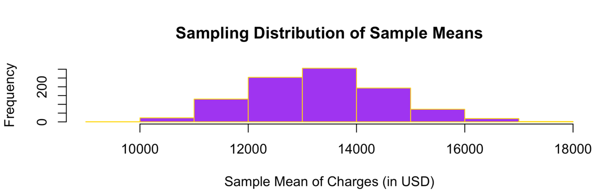
1,000 sample means, n = 100. The individual charges are lopsided; their averages are not.

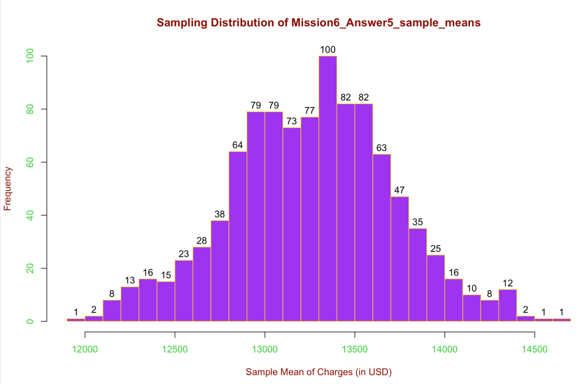
Same 1,000 means, n = 700. Same centre. A third of the width.

The centre does not move. The spread does. And the spread is what the last question was asking about, via the formula: the standard error is the population standard deviation divided by the square root of n.

Sigma is $12,105.48 and it never changes — it is a fact about the city, not about my sampling. Only the denominator moves.

You can check that against my own plots without doing any arithmetic. The n = 100 histogram spans about $7,000. The n = 700 one spans about $2,800. That is 40%, and the difference between 40% and 38% is that I am eyeballing axis labels.

Seven times the data buys you 2.65 times the precision. Not seven times. The square root is not a technicality in the formula; it is the reason data collection has diminishing returns, and it is why “just get a bigger sample” is expensive advice. I had known the formula had a square root in it. I had never once converted it into a sentence about cost.

One footnote, because it took me another pass to see it. That formula has a condition attached, and the condition is a single argument: replace = TRUE. Drawing 700 people with replacement keeps every draw independent, which is what licenses the plain σ/√n. Draw 700 of 1,338 without replacement — over half the city — and you would owe a finite population correction, the factor √((N−n)/(N−1)), about 0.69 here, because once you have taken half the town the people left over tell you something about the people you took. The assignment sidesteps that entirely. I had been carrying the formula around without the clause.

The n = 5 case, and the thing I got wrong about it

The second half of the assignment repeats everything with age instead of charges, and starts at n = 5. Five people per sample.

I have carried a summary of that plot around in my head ever since I made it, three years ago: at n = 5 the bell hasn’t formed yet, because the theorem is asymptotic. It is a tidy lesson, it is the one I would have written into this article, and I had repeated it often enough that it never occurred to me to check it. Then I opened the actual output to paste it in here.

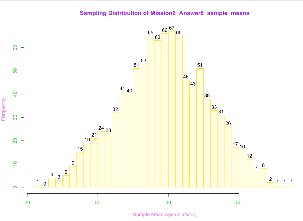
That is a bell. At n = 5.

It is symmetric, it is unimodal, it peaks within a year of the true population mean of 39.2. Nothing about it is “rough” or unformed. What is true about it is that it is wide — it runs from about 21 to about 56. Take one sample of five people and you might come away thinking the average resident is 25, or 52.

So I had been reading spread as shape. Those are two different failures and the formula separates them cleanly. Age has σ = 14.05 years, so:

• n = 5 → SE = 14.05 / √5 = 6.3 years
• n = 70 → SE = 14.05 / √70 = 1.7 years

Width is the σ/√n term, and it is large at n = 5 because √5 is 2.2. Shape is a separate question, and the answer to it depends on what you are averaging. age here runs 18 to 64 and is close to flat — roughly uniform, with a bump at the youngest end. That is about the friendliest parent a mean can have. Average as few as three draws from a flat distribution and the result already looks like a bell to the eye: the bounded ends fold inward, the middle piles up, and the shape has a name and a closed form long before it has any right to look Gaussian. By five you would have to check the tails numerically to catch the difference. charges is heavily right-skewed, which is exactly why the assignment uses n = 100 as its starting point there and n = 5 here. The switch of variable is the whole design. I had noticed it and drawn precisely the wrong conclusion from it.

The corrected lesson is more useful than the one I was carrying:

Normality is permission to use a particular set of tools. It is not a claim that your estimate is any good. The n = 5 plot has the reassuring shape and an interval six years wide; I had been reading the shape as the all-clear.

The instruction I nearly ignored

Every question in the assignment carries this note:

Each student’s R console may generate different sample means at random so the R output may vary.

I read that as an administrative kindness — don’t panic if your numbers differ from your neighbour’s. It is actually the second lesson of the exercise, stated in the marking guidance rather than the question.

My first three age sample means were 47.6, 39.6 and 44. Their average is 43.7, against a true population mean of 39.2 — off by four and a half years, which is what a standard error of 6.3 buys you when you only have three of them. Yours would be different numbers and would be wrong in a different direction. And the mean of the full thousand lands on 39.2 anyway. The individual draws are noise; the distribution of them is the signal. That the answer is stable while its components are random is the entire justification for inference from a sample — and it was sitting in a font-size-9 note about grading.

Though I should be careful about what to credit for that, because I spent a long time crediting the wrong thing. The mean of my means landing on 39.2 is not the central limit theorem. That is the law of large numbers, plus the fact that the sample mean is an unbiased estimator — average enough draws of an unbiased thing and you converge on the truth, and that would hold whatever shape the histogram came out. The central limit theorem is a claim about the shape those means take and how fast they tighten: bell, and σ/√n. Two different results, and this one exercise demonstrates both — the note about random output is the first, the histograms are the second. I had been filing all of it under one name, which is probably how the n = 5 misreading survived as long as it did. When a single label covers two ideas, you stop being able to notice which one a picture is evidence for.

What I took from it

Two things.

The first: the definition tells you what is true, and the simulation tells you what it licenses you to do. When I now put an error bar around a single sample mean, I know what that bar is a statement about — the width of a distribution I have actually watched behave, rather than a number a function handed me.

The second is less comfortable, and I only found it by going back. I had “known” this for years in a way that would have survived a quiz — and it did survive the quiz, and I still walked away with the wrong reading of my own histogram. The summary I stored was shaped like the lesson without being the lesson. There is a whole category of things I hold like that: accurate-sounding compressions with no generating procedure underneath. What protects them is that nothing ever forces a comparison. They are never wrong out loud.

A loop is a low price for finding that out. Reopening the output was cheaper still.

Thanks to whoever designed a statistics assignment where you compute the true answer first, so you can watch sampling try to reach it.

If you have a concept you’re sure you understand: can you write the smallest program that produces it — and then actually look at what it draws? I did the first part and skipped the second, and I’d have argued otherwise the day before.